Quaternions for Robotics
This article summarizes some of the practical uses and operations involving quaternions in robotic applications.
Quaternion Basics
A quaternion is defined as the following:
\[q = q_0 + \hat{i} q_1 + \hat{j} q_2 + \hat{k} q_3\]Often this is either represented in scalar-first notation or scalar-last notation:
[q_0, q_1, q_2, q_3] # scalar first
[q_1, q_2, q_3, q_0] # scalar last
But what do these values mean?
Conceptually, we can think of a rotation in 3D space as rotating some angle /$\theta/$ about a unit vector /$\vec{u}/$
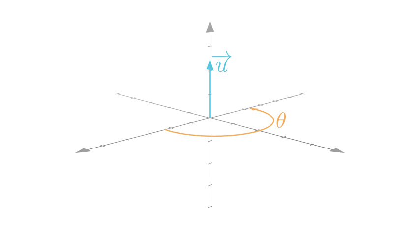
The quaternion that, when applied, performs this rotation is written as /$q/$,
\[q = cos\begin{pmatrix} \frac{\theta}{2} \end{pmatrix} + sin\begin{pmatrix} \frac{\theta}{2} \end{pmatrix} \vec{u}\]Where
\[q_0 = cos\begin{pmatrix} \frac{\theta}{2} \end{pmatrix}\] \[\hat{i} q_1 + \hat{j} q_2 + \hat{k} q_3 = sin\begin{pmatrix} \frac{\theta}{2} \end{pmatrix} \vec{u}\]Thus, we arrive at our original definition,
\[q = q_0 + \hat{i} q_1 + \hat{j} q_2 + \hat{k} q_3\]This rotation can be categorized as either an active or passive transformation. To distinguish between the two, let’s use a point as an example.
An active transformation tranforms the point in the current coordinate system to a new point in this same coordinate system.
Mathematically, we perform this active transformation by applying the quaternion as follows
\[{}^A q_2 = q \; ({}^A q_1) \; q^*\]/${}^A q_1/$ and /${}^A q_2/$ are pure quaternions that represent /${}^A p_1/$ and /${}^A p_2/$, respectively. /${}^A q_2/$ is calculated by multiplying /$q/$ with /${}^A q_1/$, then multiplying that product by /$q^*/$, the quaternion conjugate. Don’t worry if that doesn’t make sense yet; it will be made clear with examples in later sections.
On the other hand, a passive transformation expresses the same point in a different coordinate system.
Mathematically, this passive transformation is performed by applying the quaternion as follows
\[{}^B q_1 = q \; ({}^A q_1) \; q^*\]Similar to above, /${}^A q_1/$ and /${}^B q_1/$ are pure quaternions that represent /${}^A p_1/$ and /${}^B p_1/$, respectively. /${}^B q_1/$ is calculated by multiplying /$q/$ with /${}^A q_1/$, then multiplying that product by /$q^*/$
Quaternion Multiplication
But how do we actually multiply quaternions? By calculating their Hamilton product.
For two quaternions,
\[q_a = a_w + \hat{i} a_x + \hat{j} a_y + \hat{k} a_z\] \[q_b = b_w + \hat{i} b_x + \hat{j} b_y + \hat{k} b_z\]Their Hamilton product is
\[q_c = q_a * q_b\] \[q_c = c_w + \hat{i} c_x + \hat{j} c_y + \hat{k} c_z\] \[c_w = a_w b_w - a_x b_x - a_y b_y - a_z b_z\] \[c_x = a_w b_x + a_x b_w + a_y b_z - a_z b_y\] \[c_y = a_w b_y - a_x b_z + a_y b_w + a_z b_x\] \[c_z = a_w b_z + a_x b_y - a_y b_x + a_z b_w\]This is exactly what MATLAB’s quatmultiply function calculates (though the formulas at the bottom of the doc page have their elements arranged differently; if you rearrange them, you’ll see they are equivalent).
It’s important to note that qauternion multiplication is NOT commutative, i.e.
\[q_a * q_b \neq q_b * q_a\]This property is revisited later when we discuss composite rotations.
Quaternion multiplication is used often, as you will see in the sections below.
Quaternion Conjugate
If a quaternion is noted as
\[q = q_0 + \hat{i} q_1 + \hat{j} q_2 + \hat{k} q_3\]The complex conjugate of a quaternion is noted as
\[q^* = q_0 - \hat{i} q_1 - \hat{j} q_2 - \hat{k} q_3\]Note that conjugating a quaternion twice returns the original quaternion, i.e.
\[q = (q^*)^*\]Going back to our conceptual definition of a quaternion as a rotation about a unit vector /$\vec{u}/$ by a rotation angle /$\theta/$, the quaternion conjugate represents a rotation about the same unit vector, /$\vec{u}/$, with the same absolute value rotation angle, /$|\theta|/$, but in the opposite direction, /$-\theta/$. So if our original quaternion is a rotation about /$\vec{u}/$ with magnitude /$\theta/$,
\[q = cos\begin{pmatrix} \frac{\theta}{2} \end{pmatrix} + sin\begin{pmatrix} \frac{\theta}{2} \end{pmatrix} \vec{u}\]And the following trigonometric identities are true
\[cos(-\theta) = cos(\theta)\] \[sin(-\theta) = -sin(\theta)\]Then our conjugate quaternion represents a rotation about /$\vec{u}/$ with magnitude /$-\theta/$,
\[q^* = cos\begin{pmatrix} -\frac{\theta}{2} \end{pmatrix} + sin\begin{pmatrix} -\frac{\theta}{2} \end{pmatrix} \vec{u}\] \[q^*= cos\begin{pmatrix} \frac{\theta}{2} \end{pmatrix} - sin\begin{pmatrix} \frac{\theta}{2} \end{pmatrix} \vec{u}\] \[q^* = q_0 - \hat{i} q_1 - \hat{j} q_2 - \hat{k} q_3\]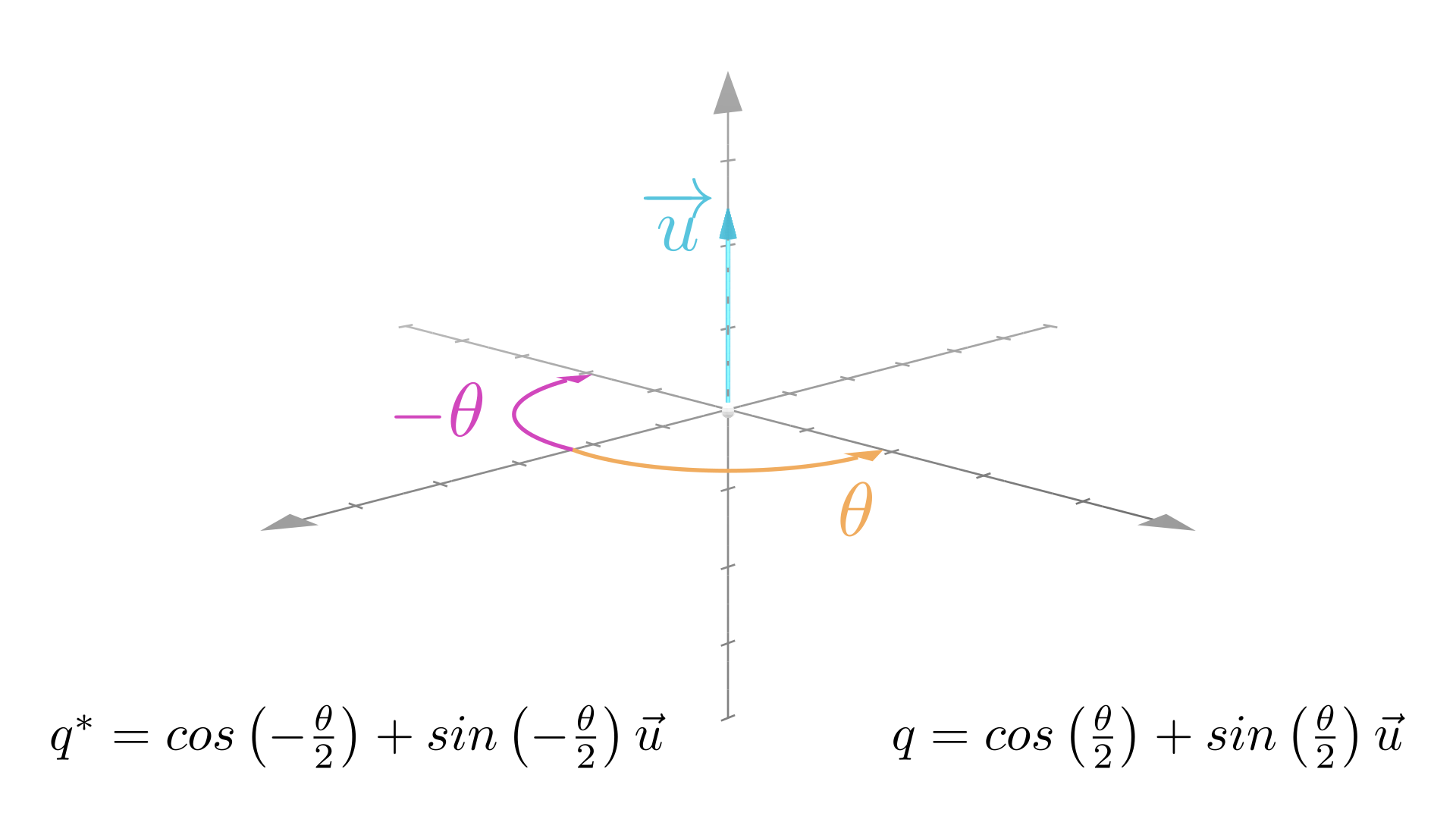
To rotate a pure quaternion, /$r_1/$, /$-\theta/$ degrees about /$\vec{u}/$, apply the complex conjugate quaternion as follows
\[r_2 = q^* \; (r_1) \; q\]Note that /${q}^*/$, /${q}^t/$, /$\tilde{q}/$, /$\bar{q}/$ may all be used to denote the complex conjugate of the quaternion.
This will come up again later…
Coordinate Frame Transformations with Quaternions
Let’s say we have two coordinate frames, /$A/$ and /$B/$.
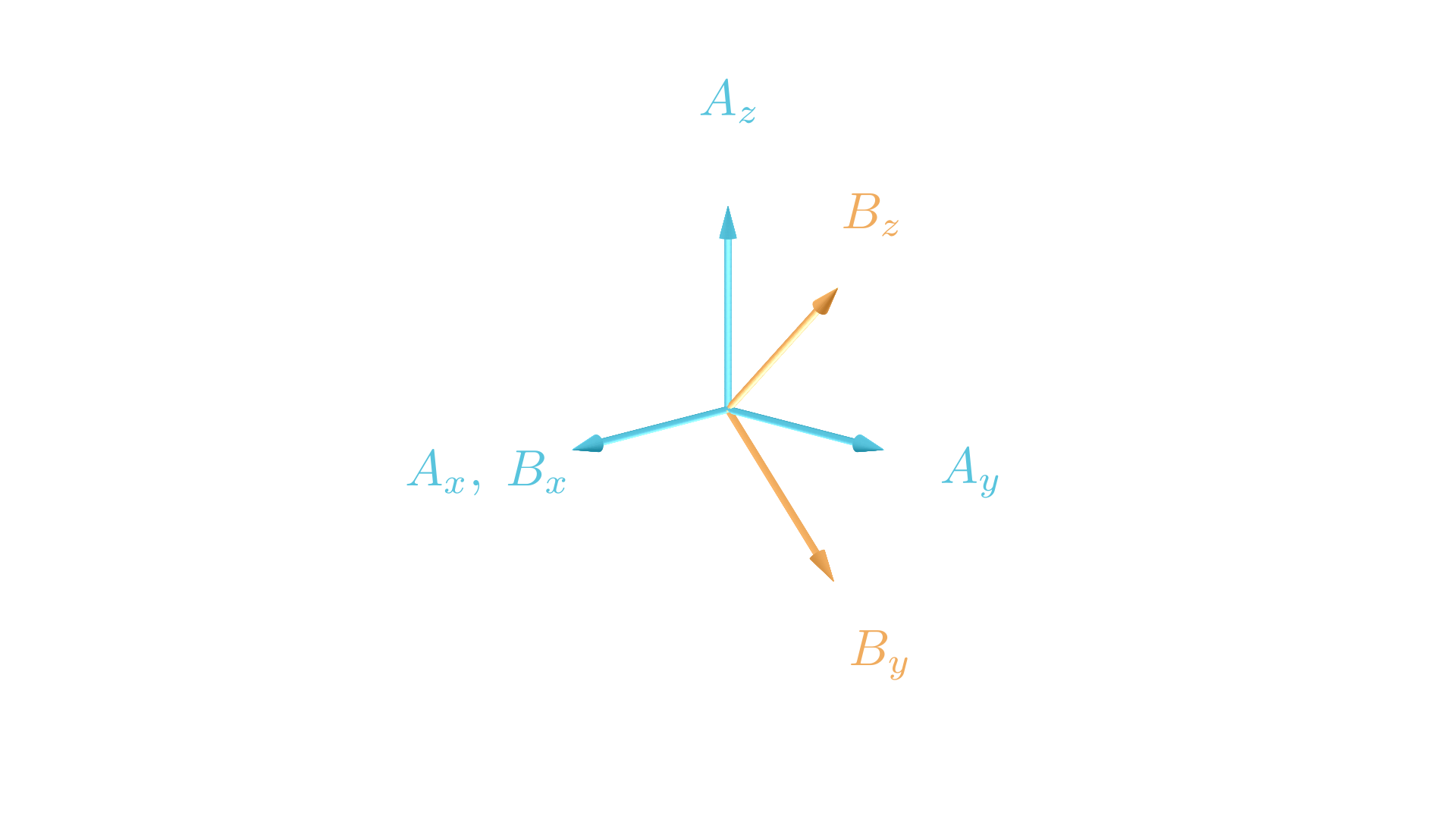
/$B/$ is rotated /$\theta = -45/$ degrees about the /$A_x/$ axis of Frame /$A/$. The quaternion describing the orientation of /$B/$ w.r.t. /$A/$ is thus
\[{}^{A}_{B}q = cos\begin{pmatrix} \frac{-45 ^\circ}{2} \end{pmatrix} + sin\begin{pmatrix} \frac{-45 ^\circ}{2} \end{pmatrix} \begin{bmatrix} 1 \\ 0 \\ 0 \end{bmatrix}\] \[{}^{A}_{B}q = 0.9239 - 0.3827 \; \hat{i}\]We can use quaternions to perform a passive coordinate transformation to take a vector expressed in /$B/$, /${}^B\vec{v}/$, and express it instead in the /$A/$ frame as follows:
-
Convert the vector to a pure quaternion, i.e. with zero scalar part (shown below with scalar-first notation)
\[{}^B q_v = \begin{bmatrix} 0 \\ {}^B\vec{v}_x \\ {}^B\vec{v}_y \\ {}^B\vec{v}_z \end{bmatrix}\] -
Perform the coordinate transformation to express the vector in the the /$A/$ frame. Note that here we use quaternion multiplication and the quaternion conjugate
\[{}^A q_v = {}^{A}_{B}q \; {}^B q_v \; {}^{A}_{B}q^*\] -
Extract the vector from the resulting pure quaternion
\[{}^A\vec{v} = \begin{bmatrix} {}^Aq_1 \\ {}^Aq_2 \\ {}^Aq_3 \end{bmatrix}\]
Running this through a numerical example: let’s say we have a vector expressed in the /$B/$ frame,
\[{}^B\vec{v} = \begin{bmatrix} 0 \\ 0 \\ 1 \end{bmatrix}\]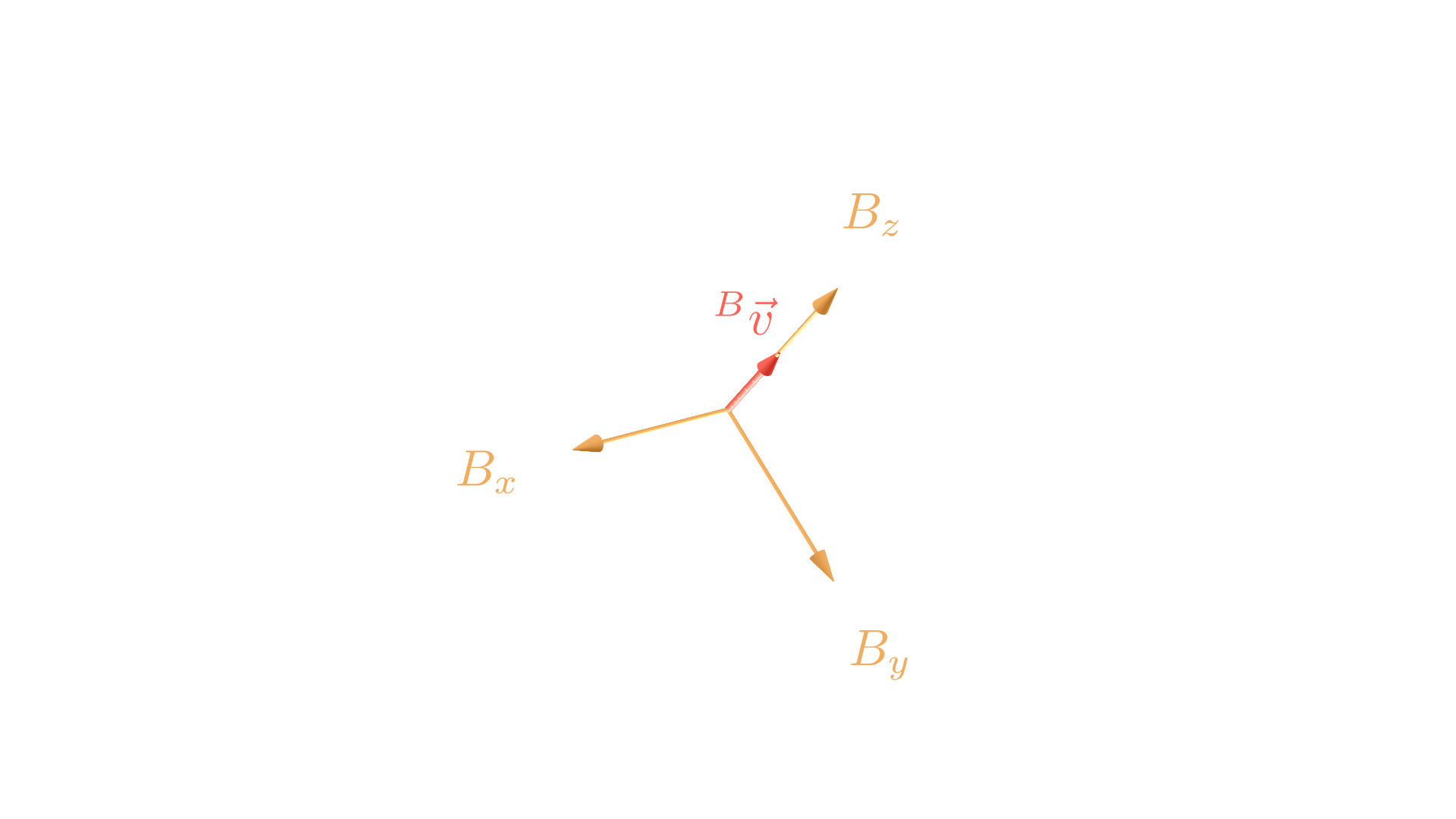
And as before, the quaternion representing the rotation of Frame /$B/$ w.r.t. /$A/$ is (in scalar-first notation):
\[{}^{A}_{B}q = cos\begin{pmatrix} \frac{-45^\circ}{2} \end{pmatrix} + sin\begin{pmatrix} \frac{-45^\circ}{2} \end{pmatrix} \begin{bmatrix} 1 \\ 0 \\ 0 \end{bmatrix}\] \[{}^{A}_{B}q = [0.9239, \;-0.3827, \;0, \;0]\]The vector can be expressed in the /$A/$ frame as follows,
>> v_wrt_B = [0, 0, 1]

v_wrt_B =

     0     0     1

>> v_wrt_B_purequat = [0, v_wrt_B]

v_wrt_B_purequat =

     0     0     0     1

>> rot_axis = [1, 0, 0]

rot_axis =

     1     0     0

>> q_B_wrt_A = [cosd(-45/2), sind(-45/2) * rot_axis]

q_B_wrt_A =

    0.9239   -0.3827         0         0

>> v_wrt_A_purequat = quatmultiply(q_B_wrt_A, quatmultiply(v_wrt_B_purequat, quatconj(q_B_wrt_A)))

v_wrt_A_purequat =

         0         0    0.7071    0.7071
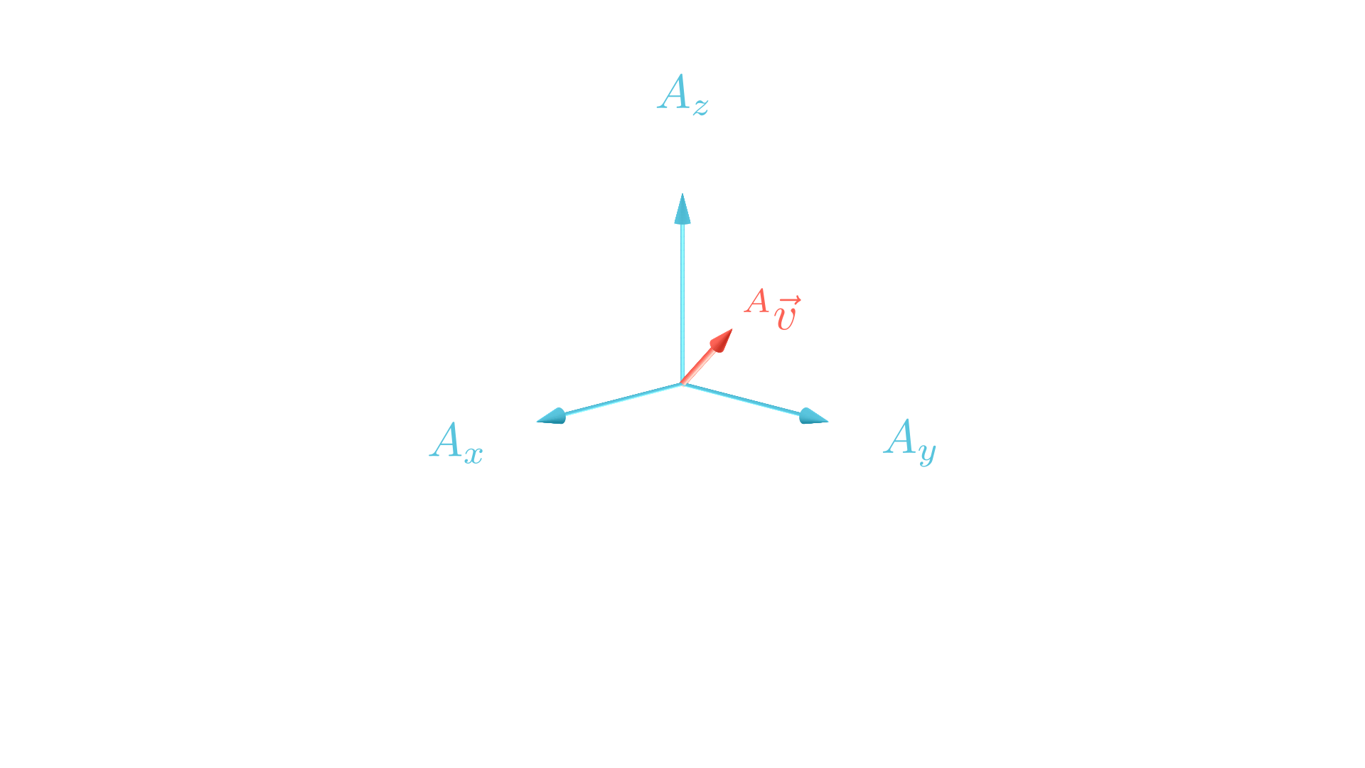
The resultant vector expressed in /$A/$ is
\[{}^A\vec{v} = \begin{bmatrix} 0 \\ 0.7071 \\ 0.7071 \end{bmatrix}\]which makes sense looking at the following picture!
Composite Rotations with Quaternions
Two successive quaternion rotations, /$q/$ and /$p/$, can be combined into one composite rotation,
\[r = p q\]where /$r/$ is the Hamilton product of /$p/$ and /$q/$. Notice that the second rotation in the sequence is left-multiplied because quaternion multiplication is not commutative. This is made clear by running through an example.
Let’s say we have a vector expressed in the /$C/$ frame, /${}^{C} v/$ (expressed as a pure quaternion), that we’d like to express in the /$A/$ frame as /${}^{A} v/$, but to get to the /$A/$ frame we have to go through the /$B/$ frame.
We can express /${}^C v/$ as /${}^A v/$ in two steps:
-
Perform a passive transformation to express /${}^{C} v/$ in the /$B/$ frame as /${}^{B} v/$
\[\;{}^B v = {}^{B}_{C}q \; {}^C v \; {}^{B}_{C}q^*\] -
Perform another passive transformation on the resultant vector /${}^{B} v/$ to express it in the /$A/$ frame as /${}^{A} v/$
\[{}^A v = {}^{A}_{B}q \; {}^B v \; {}^{A}_{B}q^*\]
Or we can do this in one step as a composite rotation, /${}^{A}_C q = {}^{A}_B q {}^{B}_C q/$
\[{}^A v = {}^{A}_{C}q \; {}^C v \; {}^{A}_{C}q^*\]Notice that because /${}^{A}_C q = {}^{A}_B q {}^{B}_C q/$ where the second rotation /${}^{A}_B q/$ is left-multiplied, these two approaches are equivalent. They both calculate /${}^{A} v/$ as follows
\[{}^{A} v = {}^{A}_{C}q \; {}^C v \; {}^{A}_{C}q^*\] \[{}^{A} v = \begin{pmatrix} {}^{A}_{B}q {}^{B}_{C}q \end{pmatrix} \; {}^C v \; \begin{pmatrix} {}^{A}_{B}q {}^{B}_{C}q \end{pmatrix}^*\] \[{}^{A} v = \begin{pmatrix} {}^{A}_{B}q {}^{B}_{C}q \end{pmatrix} \; {}^C v \; \begin{pmatrix} {}^{B}_{C}q^* {}^{A}_{B}q^* \end{pmatrix}\]This same logic applies to composite active rotations.
The Negative of a Quaternion
A quaternion and its negative represent the same resultant 3D rotation, i.e.
\[q_0 + \hat{i} q_1 + \hat{j} q_2 + \hat{k} q_3 = \\ - q_0 - \hat{i} q_1 - \hat{j} q_2 - \hat{k} q_3\]To prove this, let’s first start with an equivalent statement: a rotation by /$\theta/$ is equal to a rotation by /$\theta + 2 \pi/$
\[q(\theta, \vec{u}) = q(\theta + 2 \pi, \vec{u})\]Plugging this into our quaternion formulation,
\[cos\begin{pmatrix} \frac{\theta}{2} \end{pmatrix} + sin\begin{pmatrix} \frac{\theta}{2} \end{pmatrix} \vec{u} = \\ cos\begin{pmatrix} \frac{\theta + 2 \pi}{2} \end{pmatrix} + sin\begin{pmatrix} \frac{\theta + 2 \pi}{2} \end{pmatrix} \vec{u}\]Then leveraging two trigonometric identities,
\[cos(\alpha + \pi) = -cos(\alpha)\] \[sin(\alpha + \pi) = - sin(\alpha)\]We arrive at
\[cos\begin{pmatrix} \frac{\theta}{2} \end{pmatrix} + sin\begin{pmatrix} \frac{\theta}{2} \end{pmatrix} \vec{u} = \\ - cos\begin{pmatrix} \frac{\theta}{2} \end{pmatrix} - sin\begin{pmatrix} \frac{\theta}{2} \end{pmatrix} \vec{u}\]And finally in the familiar quaternion form
\[q_0 + \hat{i} q_1 + \hat{j} q_2 + \hat{k} q_3 = \\ - q_0 - \hat{i} q_1 - \hat{j} q_2 - \hat{k} q_3\]Sure enough, if you apply this to the example above, specifically by replacing the quaternion /${}^{A}_{B}q/$ with its negative,
\[{}^{A}_{B}q = [0.9239, \;-0.3827, \;0, \;0]\] \[\downarrow\] \[{}^{A}_{B}q = [-0.9239, \;0.3827, \;0, \;0]\]you will arrive at the same solution as in the original example. Thus, we can say that a quaternion and its negative represent the same 3D rotation.
Similarly, rotating /$\theta/$ degrees about /$\vec{u}/$ is the same as rotating /$-\theta/$ degrees about /$-\vec{u}/$. Remembering that /$cos(-\theta) = cos(\theta)/$ and /$sin(-\theta) = -sin(\theta)/$,
\[cos\begin{pmatrix} \frac{\theta}{2} \end{pmatrix} + sin\begin{pmatrix} \frac{\theta}{2} \end{pmatrix} \vec{u} = \\ cos\begin{pmatrix} -\frac{\theta}{2} \end{pmatrix} + sin\begin{pmatrix} -\frac{\theta}{2} \end{pmatrix} (-\vec{u})\]Angular Rate Calculation from Quaternions
We can calculate the angular rate command, /$W/$, that takes us from our current attitude, /$q_{est}/$, to our desired attitude, /$q_{cmd}/$ over a time step /$dt/$ as
\[2 \dot{q} {q_{cmd}}^{-1} = W\]where /$W/$ is a pure quaternion and /$q_{cmd}/$ is a normal quaternion
\[W = \begin{bmatrix} 0 & \omega_x & \omega_y & \omega_z \end{bmatrix}\] \[q_{cmd} = \begin{bmatrix} q_0 & q_1 & q_2 & q_3 \end{bmatrix}\]The equation introduced above is just a rearrangement of the following identity
\[\dot{q} = \frac{1}{2} W q_{cmd}\] \[(\dot{q} = \frac{1}{2} W q_{cmd})2\] \[(2 \dot{q} = W q_{cmd}) {q_{cmd}}^{-1}\] \[2 \dot{q} {q_{cmd}}^{-1} = W\]where /${q_{cmd}}^{-1}/$ is the inverse /$q_{cmd}/$.
We can approximate /$\dot{q}/$ as
\[\dot{q} = \frac{q_{cmd} - q_{est}}{dt}\]Thus, we have /$W/$, the angular rate command that will achieve our desired attitude, /$q_{cmd}/$
The code goes:
% differentiate quat by approximation
q_est = q_est / norm(q_est); % normalize
q_cmd = q_cmd / norm(q_cmd); % normalize
q_dot = (q_cmd - q_est)/ dt;

% calc angular rate omega = 2 * q_dot * conj(Qcmd)
w = 2*quatmultiply(q_dot, quatinv(q_cmd));
Quaternion Resources
Just some of the resources I have found helpful when learning about quaternions: